Introduction

If you've ever tried to really understand neural networks, you've probably encountered the perceptron. Maybe in a tutorial that rushed through it in five minutes, or a textbook that drowned it in notation, or a course that treated it like ancient history before jumping to transformers and diffusion models.

Here's the thing though: the perceptron isn't a stepping stone to neural networks. It is neural networks, in their simplest form. Everything else we've built since (CNNs, LSTMs, transformers) is just clever arrangements of this same basic idea.

Most explanations skip why anyone thought to build this thing in the first place. They present it as this arbitrary mathematical construct, as if a researcher just woke up one day and decided to multiply some numbers together. But the real story reveals something deeper: the perceptron was an attempt to steal computation from biology itself. Not to simulate intelligence, but to find the minimal unit of learning. What's the simplest thing that can actually get better at a task by looking at examples? That question shaped early work.

So let's start at the beginning. Not with equations or Python classes, but with the moment a psychologist in 1958 looked at a brain cell and thought he could build one with wires and motors.

The Origin Story: From Biology to Silicon

First, Let's Peek Inside The Brain

Before we get to the perceptron, we need a quick neuroscience detour. Just the essential parts.

A biological neuron is a decision-maker. It receives chemical signals from thousands of other neurons through its dendrites. The neuron doesn't treat all inputs equally: some signals get amplified (excitatory), others get dampened (inhibitory). The neuron adds everything up, and if the total crosses a threshold, it fires its own signal down the axon to the next neurons in line.

That's it. Input → weighted sum → threshold → output. This mechanism, chained together 86 billion times in your brain, somehow produces consciousness, creativity, and your ability to understand this sentence.

1943: The "What If We Built One?" Moment

Before we get to Rosenblatt and his perceptron, we need to talk about two researchers who had an even bolder idea fifteen years earlier.

Warren McCulloch (a neurophysiologist) and Walter Pitts (he was a teenager who taught himself logic) published a paper in 1943 that basically said: "neurons can be modeled as logic gates." They created the first mathematical model of a neuron. Super simple, extremely simplified. As Wikipedia diplomatically puts it, these were "caricature models" that captured one key idea while ignoring basically everything else about real neurons.

But that one idea was enough. If neurons were just biological switches that turned on when enough input arrived, then maybe, just maybe, you could build thinking machines.

1958: Enter the Perceptron

Fast forward to 1958. The Space Race is in full swing, computers still use punch cards, and Frank Rosenblatt (a psychologist at Cornell Aeronautical Laboratory) announces something that makes headlines worldwide. He hasn't just modeled a neuron mathematically. He's built one in hardware, with actual wires and motors.

The New York Times ran an article calling it "the embryo of an electronic computer that [the Navy] expects will be able to walk, talk, see, write, reproduce itself and be conscious of its existence." A bit optimistic, as it turned out.

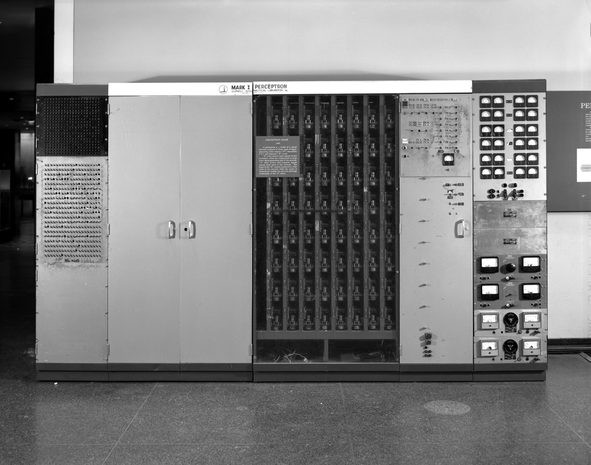
The Mark 1 Perceptron was a beast of a system. It weighed about a ton, had 400 photocells as "eyes," and used motors to physically adjust potentiometers that represented the weights.

But it could learn. Show it enough examples of letters, and it would learn to recognize them. Not because someone programmed it with rules about what makes an "A" different from a "B," but because it figured it out by adjusting those motorized weights.

If you think about it, Rosenblatt didn't just prove learning could be computed; he proved it could be mechanized. Those whirring motors adjusting potentiometers were doing something that, until that moment, only biological systems could do: learning from experience. The machine was literally rewiring itself, just more clumsily than neurons do.

The Parallel: Biology → Circuit → Math → Code → LLM

Strip away the motors and wires, and the perceptron is just math doing exactly what neurons do:

Look at that progression:

Biological: Dendrites receive signals → synaptic strengths modulate them → cell body accumulates → threshold determines firing

Conceptual: Inputs arrive → weights scale them → everything sums → activation function decides output

Mathematical: y = f(Σ(wi × xi) + b) where f is typically a step function

It's the same exact principle, just expressed in different languages. The perceptron takes inputs, multiplies each by a weight (importance), adds them up with a bias term, and decides whether to "fire" (output 1) or stay quiet (output 0).

That's it. A brain cell in 4 lines of Python. As we'll see later, there's both an intuitive and a rigorous mathematical justification for why this works.

Now that we have the intuition, let's dive deeper.

Understanding the Perceptron

Perceptron: A Geometric Intuition

Imagine you're a veterinarian with a very specific (and slightly ridiculous) diagnostic tool. You've discovered that you can tell cats from dogs using just two measurements:

• Body weight in kg (x-axis)
• Vocalization frequency in Hz (y-axis)

Dogs tend to be heavier (10-40 kg) and bark at lower frequencies (100-500 Hz). Cats are lighter (3-7 kg) and meow at higher frequencies (700-1500 Hz). Plot enough examples, and something interesting happens:

Each point represents one animal. Notice how they naturally cluster into two groups?

As they cluster into 2 groups, we should be able to separate them with one line. Here's how it looks:

Drawing a line that separates the 2 regions in 2D space

This is what the perceptron does: find that line. Given a new animal's weight and vocalization frequency, tell us which side of the line it falls on. Cat or dog. That's our ML model: a region-separating line.

But Why Do We Need a Perceptron for This?

You might be thinking: "I can see where to draw that line. Why do we need an algorithm?" This is actually the right question to ask. In 2D, with clean data, you could eyeball it. But this is where things get interesting.

Scan a single 2D slice on the left, then watch how the perceptron collapses everything onto w · x + b and reveals the per-feature contributions at the bottom. You cannot "eyeball" that in 50,000 dimensions.

The moment you move beyond toy problems, human intuition completely breaks down. Real-world data doesn't come in neat 2D packages. When you're classifying:

• Emails as spam/not spam: Hundreds of word frequencies as dimensions
• Images of handwritten digits: Each pixel is a dimension (784 for a 28×28 image)
• Medical diagnoses: Dozens of test results, symptoms, and patient history

Suddenly you're not looking for a line in 2D space. You're looking for a hyperplane in n-dimensional space, where n could be thousands. This is where math becomes almost unreasonably effective. The perceptron works exactly the same way whether it's 2 dimensions or 2,000. Same algorithm, same update rule, same convergence guarantees. The only difference is the for loop runs longer.

The Math: Which Side Are You On?

Let's get mathematical. We need to figure out: given a line and a point, which side is the point on?

Let's say we've found a separating line. In math terms, every line in 2D can be written as:

Ax + By + C = 0

Where A, B, and C are just numbers that define the line's position and angle. For example:

• 2x + 3y - 6 = 0 might be our cat/dog separator
• Points where 2x + 3y - 6 = 0 are exactly on the line
• But what about points that are NOT on the line?

Here's the interesting part: if you plug any point's coordinates into that equation, the result tells you everything:

• Ax + By + C > 0: Point is on one side (let's say "dogs")
• Ax + By + C = 0: Point is exactly on the line (confused veterinarian)
• Ax + By + C < 0: Point is on the other side ("cats")

Let me show you why this works with a concrete example:

See the pattern? We have three points with the same x-coordinate (0) but different y-coordinates:

• Point at (0, 2): Plugging in gives 2(0) + 3(2) - 6 = 0 → On the line
• Point at (0, 3): Plugging in gives 2(0) + 3(3) - 6 = 3 → Positive, above the line
• Point at (0, 1): Plugging in gives 2(0) + 3(1) - 6 = -3 → Negative, below the line

The y-coordinate increased from 1 to 3, and our equation's result went from negative to positive. That is exactly what we want the algorithm to do.

Making Predictions: The Sign Function

The perceptron's job boils down to a simple task:

1. Take a point (x, y)
2. Calculate Ax + By + C
3. Check the sign:
   • Positive → Class 1 (dog)
   • Negative → Class 0 (cat)
   • Zero → Pick a side (usually we default to one class)

In math notation:

prediction = sign(Ax + By + C)

Where sign() is:

• sign(positive number) = +1
• sign(negative number) = -1
• sign(0) = 0 (or we pick a side)

But Wait, This Is Starting to Look Familiar...

Remember the perceptron function from earlier?

And our line classification:

Look at that! They're the same thing!

• Our inputs are [x, y] (the coordinates)
• Our weights are [A, B] (the line's coefficients)
• Our bias is C (the constant term)

The perceptron isn't doing anything mysterious. It's finding the right values for A, B, and C to separate the data. The "learning" is adjusting these numbers until the line is in the right place.

Try It Yourself: The Interactive Perceptron

Now that you understand the connection that a perceptron computes Ax + By + C and checks if it's positive, let's play with one. Below is a live perceptron where:

• Inputs (x) are your coordinates [x, y] from the cat/dog example
• Weights (w) are the coefficients [A, B] that define the line
• Bias (b) is the constant term C
• The output tells you which side of the line you're on (1 for dog, 0 for cat)

Adjust inputs (your data point), weights (line orientation), and bias (line position) to control the perceptron's decision

The Activation Function: Teaching Our Perceptron to Make Decisions

So far we've been casually using phrases like "if the sum is positive, output 1" without discussing the function that makes this decision. Enter the activation function: the perceptron's decision-making personality.

Remember our basic flow: inputs → weighted sum → ??? → output.

That ??? is the activation function, and it determines how our artificial neuron responds to its inputs.

Think of activation functions like different types of judges. Here are the common ones:

1. Sign function: The harsh binary judge: you're either guilty or innocent, no middle ground
2. Sigmoid: The probability judge: "I'm 73% sure you're guilty"
3. ReLU: The optimist: only cares about positive evidence
4. Tanh: The balanced judge: considers both positive and negative equally

Activation functions are a rabbit hole we could spend hours exploring (and we will, in a future post).

Different activation functions give neurons different "personalities": decisive, probabilistic, or selective

But for the original perceptron, we're using the simplest one: the sign function.

Simple. No probabilities, no gradients, just a hard decision. This binary nature is both the perceptron's strength (clear decisions) and its weakness (can't express uncertainty). But for now, it's perfect for our cat/dog classifier.

How Perceptrons Learn

Training: Teaching a Random Line to Find Its Purpose

We don't start with the perfect line that separates cats from dogs. We start with absolute chaos: a random line that's probably wrong about everything.

Think about this for a second. The entire field of machine learning is built on this seemingly insane premise: start with random noise and nudge it toward truth. Not design it, not engineer it, just repeatedly correct its mistakes until it stops being wrong. It's like teaching someone to paint by starting with random brushstrokes and only saying "wrong" or "right" after each stroke.

Our line equation Ax + By + C = 0 needs values for A, B, and C. Since we have no idea what they should be, we just... make them up:

These numbers (A, B, and C) are our parameters (also called weights and bias). They completely define our line. Change them, and the line moves. The entire "learning" process is just finding the right values for these three numbers.

The Training Loop: Nudge, Check, Repeat

Training a perceptron is beautifully simple. Here's the entire algorithm:

1. Start with a random line
2. Show it a data point
3. If it gets it right: do nothing
4. If it gets it wrong: nudge the line toward the correct answer
5. Repeat until the line stops being wrong

That's it. No calculus, no complex optimization, just: "Wrong? Move a bit. Wrong again? Move a bit more."

Let's try this again with the animation from earlier, and also train it.

Watch the line converge, one update at a time

How exactly do we "nudge" the line?

The Update Rule: How to Nudge a Line (The Perceptron Trick)

Let's make this concrete. Say our random line encounters this situation:

• Point: (x=2, y=3) - a quiet cat
• True label: -1 (it's a cat)
• Our prediction: sign(0.73(2) - 0.41(3) + 0.22) = sign(0.45) = 1 (we predicted dog)

We're wrong. The point is actually a cat (-1) but we predicted dog (1). How do we fix this?

The perceptron uses what's often called the "perceptron trick", and it's quite simple:

• If correct: Do absolutely nothing
• If wrong: Add (or subtract) the point from your weights

That's it. When you misclassify a point, you just add its coordinates to your weights (scaled by its label):

• New A = Old A + (true_label × x)
• New B = Old B + (true_label × y)
• New C = Old C + (true_label × 1)

In our example:

• New A = 0.73 + (-1 × 2) = -1.27
• New B = -0.41 + (-1 × 3) = -3.41
• New C = 0.22 + (-1 × 1) = -0.78

And that's it. You are pulling the decision boundary toward misclassified positive examples and pushing it away from misclassified negative examples. Each mistake provides a corrective signal.

The Complete Training Algorithm (Using the Perceptron Trick)

Let's break down what's actually happening when a perceptron learns using the intuitive "perceptron trick". The algorithm maintains a "guess" at good parameters (weights and bias) and improves them one mistake at a time. As you can see, it only changes when it's wrong. When it's right, it has the confidence to do absolutely nothing.

This simple heuristic rule might seem arbitrary, but there's actually a rigorous mathematical justification for it (which we'll explore in detail below). Let's put it all together in actual code:

That's the entire learning algorithm: simple yet powerful enough to be the foundation of all neural networks.

The Clever Trick: Why y × a Tells Us If We're Right

There's a neat mathematical trick that shows up in many places in machine learning. Instead of checking if prediction != true_label, we check if true_label * activation <= 0.

Watch how the algebra works:

• If true_label = 1 (dog) and activation > 0 (we think dog), then
  1 × positive = positive ✓
• If true_label = -1 (cat) and activation < 0 (we think cat), then
  -1 × negative = positive ✓
• If true_label = 1 (dog) and activation < 0 (we think cat), then
  1 × negative = negative ✗
• If true_label = -1 (cat) and activation > 0 (we think dog), then
  -1 × positive = negative ✗

The product is positive when we're right, negative when we're wrong. This trick (multiplying by the label) turns a two-case check into a single inequality. It's one of those mathematical coincidences that's so convenient it feels like a free lunch. You'll see this pattern everywhere: in SVMs, in logistic regression, in neural network loss functions. Once you spot it, you can't unsee it.

Why Does This Update Rule Work?

When we update our weights after a mistake, we're guaranteed to do better on that same point next time. Not necessarily correct, but better. Let's see why.

Let's say we see a positive example (y = +1) but our activation is negative (a < 0). We're wrong, so we update:

• New weight₁ = Old weight₁ + 1 × x₁
• New weight₂ = Old weight₂ + 1 × x₂
• New bias = Old bias + 1

If we see the same point again, what's our new activation?

New activation = (w₁ + x₁) × x₁ + (w₂ + x₂) × x₂ + (bias + 1)
                = w₁×x₁ + w₂×x₂ + bias + (x₁² + x₂² + 1)
                = Old activation + (x₁² + x₂² + 1)

Since x₁² and x₂² are always positive, the new activation is always at least the old activation plus 1. We've moved in the right direction! We might not classify it correctly yet (if the old activation was -10, adding 1 only gets us to -9), but we're definitely closer.

Back to Simplicity: Why We'll Stick with the Perceptron Trick

We just proved that the perceptron trick (add or subtract misclassified points) is mathematically equivalent to gradient descent on the hinge loss. So should we think about perceptrons in terms of optimization, loss functions, and subgradients from now on?

The answer is: probably not, at least not for everyday use.

Yes, the formal derivation shows our simple heuristic is mathematically rigorous, it's not just a lucky guess, it's actually optimal gradient descent. But in practice, the "perceptron trick" mental model is much easier to understand and implement. You don't need to know about hinge loss, subgradients, or optimization theory. You just need to remember: "if wrong, nudge the weights toward the correct answer."

Going forward in this post, we'll continue using the perceptron trick as our mental model. The mathematical derivation gives us confidence that this simple rule is theoretically sound, but for building intuition and practical implementation, the simple heuristic wins. Sometimes the best explanations are the simplest ones that still work.

Critical Nuance #1: The Order Matters

The order you show examples to your perceptron can make the difference between learning in seconds or never learning at all.

Same data, different order: different outcomes

Imagine training on 500 cat examples followed by 500 dog examples:

• After 5 cats: "Everything is a cat."
• Next 495 cats: "Seems correct."
• First dog appears: "Wait, what?"
• After 10 dogs: "Everything is a dog."
• Next 490 dogs: "Seems correct."

By the end, your perceptron has really only learned from about 15 examples out of 1000. The rest was just reinforcement of wrong ideas.

The fix: shuffle your data. In practice, reshuffling every iteration (epoch) improves convergence and is typically up to about 2× faster on average.

Critical Nuance #2: How Many Times Should We Loop? (The Epochs Dilemma)

A hyperparameter is a setting you choose before training starts (as opposed to parameters like weights, which the algorithm learns). The most important one? How many times to loop through your data, called epochs.

• Both errors high: Underfitting (need more epochs)
• Training error near zero, test error high: Overfitting (too many epochs)
• Both errors low and stable: Just right.

The Learning Rate: How Big Should Our Nudges Be?

So far, when we make a mistake, we've been adding the full input values to our weights. But what if we only added a fraction? Enter the learning rate (α).

With learning rate, our update rule becomes:

Think of it like learning to throw darts:

• High learning rate: You drastically change your throw after each miss (might overshoot)
• Low learning rate: Tiny adjustments after each miss (might take forever to improve)

Beyond Simple Classification

Beyond 2D: When Lines Become Planes (and Hyperplanes)

So far we've been working in 2D, easy to visualize, easy to understand. But what about 3D data? Instead of a line, we get a plane: Ax + By + Cz + D = 0

The Universal Perceptron: Any Number of Dimensions

That same simple update rule works whether you have 2 features or 2,000:

Whether you're classifying images (784 dimensions for MNIST), text (thousands of word frequencies), or cat videos (millions of pixels), the perceptron uses the exact same algorithm. The only difference is the loop runs longer.

And that's the best part of the perceptron: a simple idea that scales from toy problems to real-world applications without changing its fundamental nature.

Theory and Convergence

The Convergence Theorem: Will It Ever Stop Learning?

You've been watching your perceptron adjust its weights, iteration after iteration. But here's a question that should bother you: will it ever stop? Or will it keep tweaking forever?

This isn't just philosophical anxiety. If the perceptron never settles on a solution, we can't actually use it. We need to know: given linearly separable data, will the perceptron eventually find a separating line and stop updating?

The answer is yes, and the proof is one of the more elegant results in machine learning. What makes it great is that it proves convergence without ever constructing the solution. It's like proving that someone will eventually reach the top of a mountain without knowing which path they'll take.

What Does "Convergence" Mean?

Convergence happens when the perceptron makes a complete pass through all training data without making a single update. Every point is classified correctly. The weights have settled into their final values. Learning is done.

Geometrically, convergence means we've found a hyperplane that puts all positive examples on one side and all negative examples on the other. No more mistakes, so no more updates.

But there's a catch. Let me show you two scenarios:

The perceptron on the linearly separable data finds a solution and stops. The other one keeps changing its mind forever. The difference? The data on the first graph is linearly separable: a straight line can divide the classes. The data on the second (XOR pattern) isn't, so no straight line will ever work.

So our first requirement for convergence: the data must be linearly separable. If it's not, the perceptron will update forever, like Sisyphus pushing his boulder up the hill only to watch it roll back down.

The Margin: Measuring How "Easy" a Problem Is

Not all linearly separable problems are created equal. Some are easy, where the classes are far apart with lots of room for the boundary. Others are hard, where the classes nearly touch, and you need to thread the needle perfectly.

We measure this difficulty with the margin (denoted γ, gamma). The margin is the distance from the decision boundary to the closest data point. Think of it as the "safety buffer" or cushion of empty space around your separating line.

To understand margin mathematically, let's break it down:

For a single point: The signed distance from a point (x) with label y to the hyperplane defined by weights w and bias b is:

signed distance = y × (w·x + b) / ||w||

Where:

• y is the true label (+1 or -1)
• w·x + b is the raw activation (positive on one side, negative on the other)
• ||w|| is the length of the weight vector (for normalization)
• The multiplication by y makes the distance positive when correctly classified, negative when misclassified

For a dataset: The margin is the minimum of these distances across all points:

margin(D, w) = min(all points) [y × (w·x + b) / ||w||]

This tells us: "What's the closest any point gets to the boundary?" If even one point is misclassified, the margin becomes negative.

The best possible margin: For a dataset D, we define its margin γ as the best margin any separator could achieve:

γ = margin(D) = max(all possible w) [margin(D, w)]

If the data isn't linearly separable, this maximum doesn't exist (no valid separator), and there's no positive margin.

The Proof: Why the Perceptron Must Converge

The convergence proof is sneaky and smart. We're going to set up a race between two quantities that grow at different speeds, and show that one can't keep up with the other forever.

Here's the setup: imagine you're tracking two things as the perceptron learns. One quantity grows linearly (like k, 2k, 3k...) with each mistake. Another quantity grows sublinearly (like √k) with each mistake. These two quantities are also constrained to satisfy an inequality. Eventually, the linear growth will violate this inequality unless the mistakes stop.

What This Really Means

The bound tells us three crucial things:

1. Convergence is guaranteed: The perceptron can make at most R²/γ² mistakes on linearly separable data. After that, it must have found a separating hyperplane.

2. Larger margins → faster convergence: If the classes are well-separated (large γ), we learn quickly. If they're barely separable (tiny γ), we might need many updates.

3. Data scale matters: If we scale all our data points by 10, R increases by 10, but so does γ. The bound R²/γ² stays the same. This scale invariance is useful.

But here's what the proof doesn't tell us:

• Which separator we'll find: The data might be separable with margin 0.9, but the perceptron might find a boundary with margin 0.00001. It just needs to find some separator, not necessarily the best one.
• How to check if data is linearly separable: If it's not, the perceptron will run forever. There's no general efficient algorithm to check separability beforehand, you just have to try and see if it converges.
• The exact number of iterations: The bound R²/γ² is often pessimistic. Real convergence is usually much faster because the bound assumes worst-case behavior at every step.

The convergence theorem is like a warranty: it guarantees the perceptron will work on linearly separable data, but doesn't promise it'll find the best or prettiest solution. For that, we need fancier algorithms (which we'll see later).

But for a simple algorithm from 1958, a mathematical guarantee of convergence is pretty remarkable. It's why the perceptron remains a cornerstone of machine learning theory, even as we've moved on to deeper and more complex models.

Modern Perceptron Variations

Let's look at some practical improvements to the basic perceptron that address its limitations.

The vanilla perceptron we've been working with has a weakness: it's biased toward recent examples. This makes it vulnerable to a failure mode worth understanding. Fortunately, there are two clever fixes: one beautiful but impractical (voted perceptron), and one slightly less beautiful but actually usable (averaged perceptron).

The Late-Update Problem

The vanilla perceptron is biased toward recent examples. If your perceptron correctly classifies 9,999 examples, then misclassifies the 10,000th (maybe it's noisy or mislabeled), that single update overwrites weights that were 99.99% accurate.

This is the perceptron's recency bias. The last example to cause an update has massive influence, regardless of how well the previous weights performed.

The Voted Perceptron: Democracy for Hyperplanes

The voted perceptron solves this by keeping every weight vector the algorithm ever considers, along with how long each one "survived" before being updated. At test time, each historical weight vector votes on the classification, weighted by its survival time.

Here's the idea: if a weight vector classified 500 examples correctly before finally making a mistake, it gets 500 votes. If another weight vector got updated immediately, it gets just 1 vote.

There's solid theory proving the voted perceptron generalizes better than vanilla. But it's completely impractical.

If your perceptron makes 1,000 updates during training, you need to store 1,000 weight vectors. Prediction becomes 1,000× slower because you need to compute 1,000 dot products instead of one. For high-dimensional data, this quickly becomes absurd. Imagine storing 1,000 copies of a million-dimensional weight vector.

The Averaged Perceptron: The Practical Compromise

The averaged perceptron takes the voting idea and makes one crucial simplification: instead of letting each weight vector vote, we just use their average.

The mathematical trick here is subtle but clever:

See what happened? We moved the sign function outside the sum. This changes the semantics (averaging votes vs. voting on averages) but in practice works almost as well. The benefit is that now we can precompute the averaged weight vector:

But wait. This seems to require updating the averaged weights on every example, even correct ones. That is wasteful!

Here's the clever trick used in practice:

The math here is subtle but clever. By keeping track of when each weight was added and scaling by the counter, we automatically compute the average without updating on every example. It's one of those algorithms where you need to work through the algebra to believe it actually computes the right thing.

Empirical Comparison

Here's how these three variants typically perform:

The bottom line: Always use the averaged perceptron. The tiny computational overhead gives you significantly better generalization. With early stopping (halt when validation accuracy plateaus), it's remarkably effective: simple to implement, fast to run, and competitive with fancier algorithms.

Think of it this way: vanilla only remembers the last lesson, voted remembers every lesson perfectly (expensive), and averaged maintains a running wisdom without the storage cost.

Limitations and Legacy

The XOR Problem: When Lines Aren't Enough

The perceptron has one fatal flaw that almost killed AI research: it can only draw straight lines.

This sounds trivial until you realize that some of the simplest real-world patterns need curves.

The Limitation That Changed History

Consider this simple real‑life scenario: A teenager wants to go on a trip with friends. Here's how parent permissions work in this household:

• Both parents say NO → trip denied
• One parent says YES, the other says NO → they negotiate and compromise: trip allowed
• Both parents say YES → they get overexcited and turn it into a family trip instead. Solo trip denied

The "Trip allowed" outcomes sit on opposite corners. The "Trip denied" outcomes sit on the other corners. This checkerboard pattern is XOR (exclusive‑or), and no single straight line will ever separate it correctly.

This isn't a contrived mathematical curiosity. Many everyday situations follow this "disagreement = yes" pattern:

• Solo trip allowed only when parents disagree (they compromise)
• Outfit works when you pick jacket OR umbrella, but not both (you'd be overdressed)
• Coffee tastes right with milk OR sugar, but not both (too rich) or neither (too bitter)

The First AI Winter: Death by XOR

In 1969, Marvin Minsky and Seymour Papert published a book called "Perceptrons" that proved mathematically what we just saw visually: perceptrons cannot learn XOR. The proof was elegant and correct.

The impact was significant. Funding decreased, and many researchers shifted away from neural networks. The field entered what we now call the "First AI Winter."

Notably, the same book explained that multilayer perceptrons can solve XOR, but training them was considered computationally intractable with the hardware of the time.

This is a pattern in AI: we overestimate how hard things will be computationally: the "intractable" multilayer perceptron training that Minsky worried about? Your laptop today can do millions of them per second.

The perceptron can't solve XOR with a single line. But what about two lines? Or better yet, what if we stack perceptrons?

Interestingly, Minsky/Papert acknowledged this, but dismissed it thinking it would be computationally intractable.

This is the birth of neural networks: just perceptrons feeding into other perceptrons. But it took until the 1980s for this idea to gain traction, and another few decades to become deep learning.

The Perceptron's Legacy

After thousands of words, the perceptron boils down to four steps:

1. Take inputs
2. Multiply by weights
3. Add them up (plus bias)
4. Output 1 if positive, 0 if negative

A weighted sum and a threshold. You can explain it in a few minutes.

Yet this simple operation is the atomic unit of artificial intelligence. Every large language model, every image generator, every game-playing AI, they're all vast networks of this same basic operation. GPT isn't doing anything fundamentally different from Rosenblatt's 1958 machine. It's doing it a trillion times in parallel with better organization, but the core computation remains unchanged.

The perceptron reveals something about intelligence: maybe it isn't about complex reasoning units but simple units, properly connected, at massive scale. A single perceptron can only cut space with a straight line. But compose enough straight cuts and you can carve any shape. Stack enough simple decisions and you get judgment. Chain enough thresholds and you get thought; then further along? abstract thought, and so on.

Why This Still Matters

In an era of trillion-parameter models and transformer architectures, why examine something from 1958 that can't even solve XOR?

Because every breakthrough in deep learning (backpropagation, convolutions, attention mechanisms) is fundamentally about organizing perceptron-like units in clever ways. The operations evolved slightly. We use ReLU instead of step functions, softmax for multiple outputs. But the core principle persists: simple units, weighted connections, patterns learned from data.

The perceptron is like the transistor of intelligence. Sure, your CPU has billions of transistors arranged in incomprehensibly complex patterns. But crack it open and study any single gate, and you'll find the same simple switch invented decades ago. The complexity emerges from the arrangement, not the component.

Final Thoughts

The perceptron is the simplest unit that exhibits the behavior we care about in neural networks. Understanding it gives you the foundation for everything that came after, from CNNs to transformers.

When the math gets dense and the implementations complex, you can always trace it back to this: inputs, weights, sum, threshold. Everything else is billions of these decisions, orchestrated in different ways.

References and Further Reading

• Smithsonian National Museum of American History, Electronic Neural Network, Mark I Perceptron
• Towards Data Science, Explain like I'm five: Artificial neurons
• Wikipedia, Artificial neuron
• Frank Rosenblatt, The Perceptron: A Probabilistic Model for Information Storage and Organization in the Brain
• Karthik Vedula, Visualizing the Perceptron Learning Algorithm
• Hal Daumé III, A Course in Machine Learning - Chapter 4: The Perceptron